
This article was originally posted directly on my Linkedin profile / articles section.
A few months ago, I had an interesting conversation regarding the usage of analytics in finance with someone working in a German DAX-listed company which grows through M&As.
When it comes to ompany valuation, one of the method which comes back is performing a company valuation using Discounted Cash Flows method and a Monte-Carlo simulation to assess its value.
Wait, company valuation, ok, but what is a Monte-Carlo simulation?
According to Investopedia:
The Monte Carlo method is a stochastic (random sampling of inputs) method to solve a statistical problem, and a simulation is a virtual representation of a problem. The Monte Carlo simulation combines the two to give us a powerful tool that allows us to obtain a distribution (array) of results for any statistical problem with numerous inputs sampled over and over again
In other words, this has to do with sensitivity analysis: instead of having a simple and basic “low / medium / high” scenarii kind of model which one would traditionally build on Excel, a Monte-Carlo simulation will use thousands of variations of the key model’s drivers to generate a fair price for the company.
Monte-Carlo simulations allow to go beyond deterministic models and inject hazard and stochastic into the models.
When you assess the financial value of a company, there are indeed many random factors which can have an impact on the final company valuation. Revenue can grow at a stronger pace than expected, EBITDA can grow slower than expected, net working capital can also follow another path and so on.
Objectives
Step by step, we will assess the value of fictive company, using the DCF methodology and then apply the Monte-Carlo simulation to come, not to a single price for the company, but get a low / high price based on 10,000 simulations. This will factor in the randomness we observe in reality and will provide a more robust company valuation.
We’ll use a the financial data of a virtual company to do so and here are the steps we’ll follow:
- We’ll start by building on Excel the Free Cash Flow on the projected 5 years.
- Using the YoY Sales growth as an example, we’ll build a normal distribution to show how this will be used in the Monte-Carlo simulation
- We’ll migrate the Excel model to a Python script with hard-coded values just to replicate the correct model to work with.
- We’ll transform and upgrade the script to run the Monte-Carlo simulation and get a fair range of price for the company
Disclaimer
This post is purely educational and does NOT aim at giving any recommendation whatsoever regarding business. It’s focusing on showing some Python technical possibilities. You may feel free to replicate and improve the code below but I already DECLINE in advance all responsibilities. The below is only my own and does NOT reflect in any case my employer.
Step 1: Building a simple model on Excel
I built this simple model to project the Free Cash Flows of the fictive company for the next 5 years. It’s combining elements from the P&L and the balance sheet to calculate the free cash flow (=the cash which remains to pay investors and Debitors).
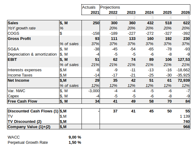
This simple model gives a valuation at $968M. The FCF model is somewhat classic, we start by the net income, re-integrates the Interests expenses, the depreciation & amortization and then we withdraw the change in net working capital and the capital expenditures. Cash flows are then discounted according to the weighted averaged cost of capital. Terminal value is valued using the perpetual growth rate and the WACC, and is also discounted with the Y5 discounted factor rate.
This model is however too rigid as it assumes :
- A flat YoY sales growth at +20%
- A flat EBIT / Sales ratio at 21%
- A constant YoY NWC variation at -1.2% of Sales
- And Capex being the same than the D&A (company invested as much as the depreciation of its assets).
A ‘classic’ analysis would establish 3 hypothesis (low, medium, aggressive) to try to assess the value, but we will go beyond and will run 10,000 simulations to come to a fair range of price for the company’s worth.
We’ll work on these ratios and use them in the Monte Carlo simulation, but first, let’s have a look at what it could look like if we make these ratios less “rigid”.
Step 2: Applying a normal distribution for the key drivers
Based on the model above, the key drivers of the model we’ll want to play with will be:
- Sales YoY growth rate (%) (which we’ll use below as an example)
- COGS as percentage of Sales: What if the company manages to negotiate lower prices from its suppliers or, on the contrary, what if the price of the raw material increases?
- SG&A as percentage of Sales (this integrates fixed and semi-fixed costs, but we’ll simplify it here and assume SG&A to be a growing function of Sales): restructuring, headcounts reduction or increased marketing sales to win market shares?
- Interest expenses
- Depreciation & amortization as % of Sales and a ratio Capex / D&A
- YoY variation in NWC
Let’s consider the sales YoY growth rate as an example.
We assumed earlier sales to grow on constant average at 20% year over year. We’ll make this growth rate change and we’ll assume a normal distribution at +/- 2%.
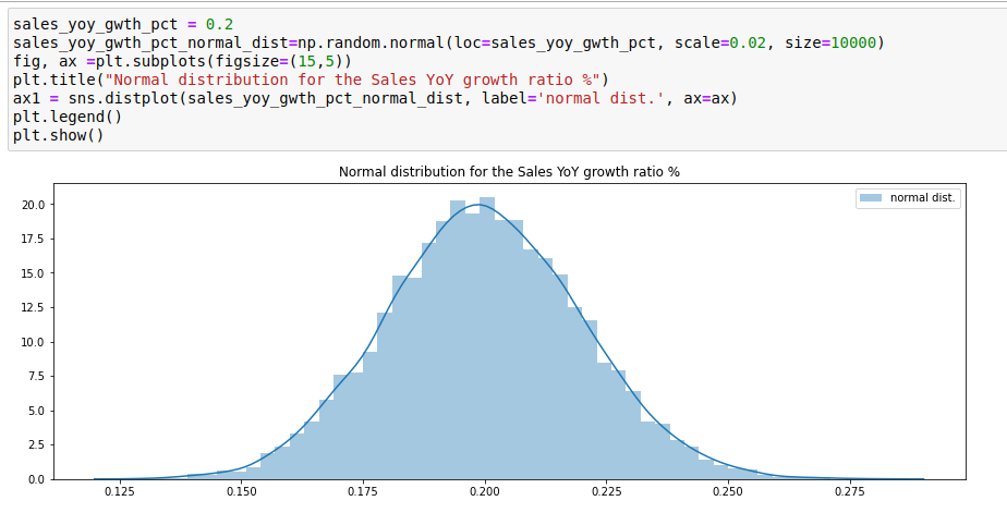
Let’s detail it. We applied a standard deviation of +/-2 ppts on the 20% growth announced.
We indeed don’t know if the sales growth will be constant at +20% (which corresponds to the mean on the x-axis) as it might be higher than expected or less but we do think that 20% is a fair assumption to start with. So as of now, ~ 68% of the sales growth values we will use in this Monte-Carlo simulation as an input variable will be between 18% and 22%.
The ~ 32% remaining will be higher than 22% of less than 18% sales YoY growth, which will allow to stress test the model with more extrem values. These extreme growth values will also be factored-in the model, but in fair proportion.
We created 10,000 values for the sales growth in just 1.66 milliseconds and now we have a typical Gaussian curve.
All the drivers mentioned previously will go through the same process and be used as inputs in our EV via DCF model.
Step 3: migrating the DFC Excel-based model to a Python script
But first, let’s migrate the Excel to a V1 Python script.
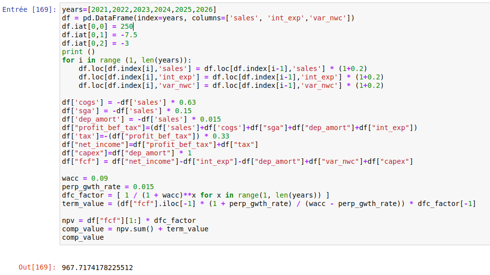
That’s good, we managed to replicate the Excel: the final output is equal to $967.7M, which is the result we expected for the company valuation.
It’s based on a single DataFrame, including all the 1+5 years projected, which has 1 column per metric.
However, the script doesn’t look great (we can say ugly):
- It’ s hard-coded and not scalable at all
- the script has no function nor class
- as it is the script requires loop to run the 10,000 simulations.
Indeed, if we want to run 10,000 simulations, we’ll need to do it through a loop and build 10,000 DataFrames.
Step 4 : Running the Monte Carlo simulation
Similar to step 2, we’ll (I) set a value for the main drivers and (II) add a standard deviation to calculate the normal distribution.
Hypothesis: Sales growth will be growing at 20% (mean) with +/- 2ppts variations, COGS at 63% of sales at +/- 1.5ppts (some years growing more, some years less), SG&A at 15% with +/- 1ppt (since this is more in-control of the company), and so on for the other drivers we identified. Remember that values going beyond these standard deviations will be also factored-in, which is great!
In terms of code, I combined the previous one and re-used some part of the code found on this post; especially the fact of leveraging the numpy matrix to improve performance, and transformed it to make it more scalable building a class.
The version below definitely looks better as :
- It’s now using a proper Class (object oriented programming) which makes it scalable: quite convenient if you need to embed it into another program.
- Numpy array make it super fast to compute: the below script runs 10,000 simulations in just 20.6 milliseconds (!). To do so, the script will create several matrix of 5 rows and 10,000 columns each (!).
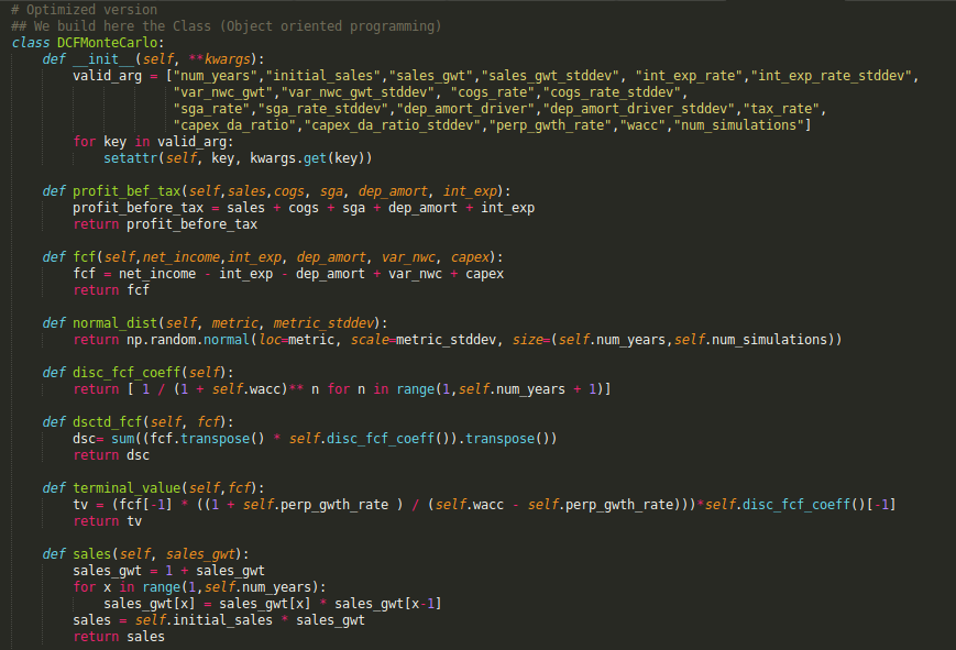
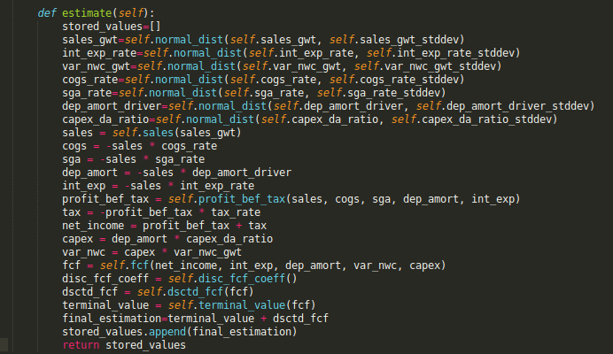
Now, to use this class, we just to enter a few parameters, easy to tune, in a dictionary format. Any JSON feed could also be provided as input (which makes it possible to evaluate literally companies by batches).
This is how I instantiated the class:
params= {
"num_years":5,
"initial_sales" : 250,
"sales_gwt":0.2,
"sales_gwt_stddev":0.02,
"int_exp_rate":0.03,
"int_exp_rate_stddev":0.005,
'var_nwc_gwt':0.8,
"var_nwc_gwt_stddev":0.02,
'cogs_rate':0.63,
"cogs_rate_stddev":0.015,
'sga_rate':0.15,
"sga_rate_stddev":0.01,
"dep_amort_driver":0.015,
"dep_amort_driver_stddev":0.001,
'capex_da_ratio':1,
"capex_da_ratio_stddev":0.01,
'tax_rate':0.33,
"perp_gwth_rate":0.015,
"wacc":0.09,
"num_simulations":10000
}

company_value = DCFMonteCarlo(**params)
value_range = company_value.estimate()
plt.figure(figsize=(13,5))
plt.title("Company valuation price range | Monte Carlo simulation with 10,000 runs")
plt.hist(value_range,  color="orange", bins=50, )
plt.show()
Finally, we get what we wanted: a fair price range of the company value with more than 10,000 simulations!
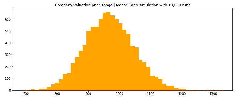
After 10,000 simulations, we see that the fair price of the company is most likely to be somewhere between $900M and $1,050M (by looking at the values located on the x-axis which have the highest frequencies).
Wait: visual is nice, but not very precise.
To get access to the data, we can use pandas get detailed information:
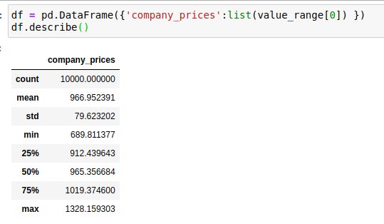
We indeed get the 10,000 simulations, which corresponds to the row “count”. The minimum is $689M (extreme low) and the maximum values the company at $1,328M (extreme high).
And now the final:
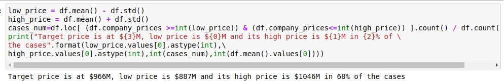
Located at 1 standard deviation of the mean (= ~ 68% of all the simulations) the price of the company is now between $887M and $1046M.
Conclusion
We estimated the price of the company to be likely at $968M in step 1. The stochastic approach via a Monte-Carlo simulation gives the price to be between $887M and $1046 after having injected 10,000 random hypothesis following a normal distribution on Sales growth, cost of goods sold, selling general and administrative, interest expenses, capex, depreciation & amortization, change in net working capital.
This approach can be replicated in almost all the business cases where we want to inject some uncertainty to get a fair range: consumers analysis, pricing analysis, input commodities prices estimations (E.g. cotton price in the fashion industry) having a strong impact on P&L
Some of the sources I used to help me:
- https://www.investopedia.com/terms/f/freecashflow.asp#mntl-sc-block_1-0-28
- https://www.wallstreetprep.com/knowledge/dcf-model-training-6-steps-building-dcf-model-excel/#:~:text=The%20DCF%20model%20estimates%20a,capitalization%20of%20approximately%20%24909%20billion.
- https://www.toptal.com/finance/financial-forecasting/monte-carlo-simulation
- https://tykiww.github.io/2018-07-05-MC-DCF/
- https://www.sharpsightlabs.com/blog/numpy-random-normal/
- https://stackoverflow.com/questions/20763012/creating-a-pandas-dataframe-from-a-numpy-array-how-do-i-specify-the-index-colum